Need to inject a custom signal into your simulation? CircuitLab has long allowed piecewise linear and piecewise step sources, but we've now added a CSV source to the toolbox. You can now paste in a larger CSV file of (time,voltage) pairs, one per line, and the simulator will use your input for simulation.
Our first example is a multilevel inverter with a piecewise-step sinusoidal-like signal, and applied low-pass filtering:
Our second example is a simple switching power supply with a edge-defined gate drive signal and a digital inhibit feedback loop:
Try out these simulations and double-click the CSV sources to look at their contents!
Our friends at the electronics component search engine Octopart have launched a new crowd-funded project: a Pocket Electronics Reference PCB. This credit-card-sized, full-color PCB fits in your wallet and contains resistor color codes and surface-mount footprints.

Watch the video and order yours today: http://www.crowdsupply.com/octopart/pocket-electronics-reference-pcb
A version of this article also appeared on EDN.
As general-purpose simulation software, CircuitLab has users who run a wide spectrum of circuit simulations. Our simulator must attempt to handle any circuit users choose to analyze. We found that a large class of simulations were failing because the system of equations was numerically ill-conditioned and couldn’t be solved numerically within the normal 64-bit floating point range, even though the circuit was completely valid. We solved a significant array of DC and transient convergence issues by extending the numerical precision of the floating point number types within the core of our solver code beyond the 64-bit “double” type available natively within Javascript.
The CircuitLab community ran more than half a million simulations last month. Each one involved constructing tens, hundreds, or even thousands of simultaneous, highly nonlinear, strongly coupled differential equations, which are repeatedly linearized and solved iteratively. Last month alone, our software constructed and factored more than 600 million matrices, and solved those factored systems more than 1.6 billion times.
However, some simulations were failing to converge, which caused a variety of problems from slow simulations to complete solver failures. When we inspected the systems generating these failures, they were well defined, by which we mean that any proficient high school math student could have computed the correct solution. But the numerical methods in the solver could not!
And here’s the core of the problem:
1 + 1e-16
Try computing this sum in your favorite scripting language: Python, Ruby, PHP, Javascript, etc. The result is simply:
1
when, to any high schooler (not aware of the limited precision of floating-point datatypes), the answer should of course be:
1.0000000000000001
This truncation to 1.0 happens because all of these languages use a standard “double precision” 64-bit floating point number to represent real numbers internally, which is capable of only about 16 significant decimal digits of storage, and must truncate the rest between operations. It’s like working on a calculator that only has room for 16 digits.
How much could this tiny difference make? One part in 10^16? Impossible for this to become an issue, right? Typically, that’s exactly right -- no real difference at all.
But the real problem begins here:
1 + 1e-16 + -1
which is evaluated as
((1 + 1e-16) + -1)
= (1 + -1)
= 0
That’s a zero that gets inserted in an equation where there really ought to be a 1e-16. And in solving equations, of course, zeros as coefficients can be quite a scary thing!
This truncation is particularly troublesome and elusive because the result depends on the order that we perform the addition:
1 + 1e-16 + -1 = ((1 + 1e-16) + -1) = (1 + -1) = 0
1e-16 + 1 + -1 = ((1e-16 + 1) + -1) = (1 + -1) = 0
1 + -1 + 1e-16 = ((1 + -1) + 1e-16) = (0 + 1e-16) = 1e-16
In this case, the only way to get the correct result is for the smallest quantity to be the last. Limited-precision data types makes addition, normally a commutative operator, into a not-always-commutative one!
These kind of operations happen in the course of LU factorization, when a matrix A is factored into separate lower and upper triangular parts to satisfy P*A=L*U. Just as in Gaussian elimination, rows of the matrix A are added or subtracted from other rows in order to clear particular entries, and this set of steps is recorded in the L and U matrices.
In an infinite-precision world, LU factorization does not have the ability to destroy information from the original matrix A. But in a limited-precision numerical implementation, it does! This brings us to the concept of a matrix’s condition number, which roughly speaking has to do with the range of quantities present with the matrix. As a very rough heuristic, one can begin to “eyeball” the condition number of a matrix by looking at the largest ratio of largest to smallest non-zero absolute values within any row or column of the matrix. An “ill-conditioned” matrix has condition number much greater than one, and as the condition number approaches the precision of the floating point data storage, more information can be lost during matrix operations.
In electronics, it’s normal to encounter a very wide range of numbers, from picofarads (10^-12), to megaohms (10^6) in common practice, already a range of 10^18 which exceeds the 16-digit precision of a double floating point type. And internal nodes within a simulation can extend several orders of magnitude beyond that range. Even within only a single quantity like current in Amperes, it’s possible to have both hundreds of amps (10^2) and tens of femtoAmps (10^-14), for example in different branches of a switching-dominated circuit. This alone doesn’t guarantee any numerical issues, because heuristics for ordering rows and columns, heuristics for pivot selection, and numerical preconditioning can adjust the structure of the problem to alleviate these issues in many circumstances. However, the fact that the simulations are completely user-specified means that sometimes, these issues do arise.
For example, try simulating this simple diode circuit in your own simulation software:
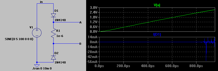
In this example from another simulation engine, a simple diode circuit easily analyzed by inspection faces serious convergence issues, taking hours and hours to simulate, and displaying noisy currents millions of times larger than would be seen in reality. Does your software do this?
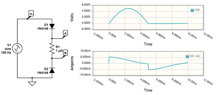
In CircuitLab, with the new extended precision numerical core we’ll describe below, this circuit and others simulates quickly and correctly in milliseconds (try it instantly!):
At CircuitLab, we solved this class of convergence issue by using a “double-double” numeric type, which uses a combination of two 64-bit doubles to represent a single extended-precision number. This is a well-known concept that’s been available since the 1960s, but CircuitLab is the first circuit simulation software available to make use of extended precision to provide better convergence.

A “double-double” represents a floating point number X = Xhi + Xlo, where Xhi and Xlo are both native 64-bit doubles, and where abs(Xhi) > abs(Xlo). In fact, Xhi and Xlo are split to represent non-overlapping ranges of precision. By using two floating point numbers, existing CPU built-in 64-bit floating point operations can be used for speed, but extended near-128-bit precision can result. Instead of 16 significant decimal digits, we now have about 32 decimal digits to work with -- a significantly expanded dynamic range. Addition, subtraction, multiplication, and division of double-double types can each be implemented with just about 10 to 20 normal double floating point operations.
Here are a few excellent references for algorithms to understand and implement double-double operations: (1, 2, 3).
While it sounds like a significant overhead to move from 1 floating point operation to 10-20, they are all compact functions requiring only a small set of registers written in a non-branching way, so they’re extraordinarily speedy on a modern CPU. We measured less than 3% slowdown within a typical well behaved circuit simulation. And because the extended precision solves so many convergence issues, our overall CircuitLab simulation test set actually runs 20% faster!
CircuitLab’s new simulation engine is now available, and we’re happy to announce what we believe is the world’s first extended-precision general purpose circuit simulation software. We’re working hard to eliminate the pain points that keep engineers from making better use of numerical simulation, from the GUI to the underlying numerical representations, and are working to extend the capabilities of our software day by day. In the coming years, we have no doubt that other simulation engine developers will follow us into the era of high-precision circuit simulation.
CircuitLab is an in-browser schematic capture and circuit simulation software tool to help you rapidly design and analyze analog and digital electronics systems.