Programming mathematical software with complex numbers, where each numeric value has a real component and an imaginary component, can be complicated. As requested by our users, CircuitLab’s circuit simulator engine now tracks a third component for each complex-valued circuit variable (i.e. voltage or current in a frequency domain simulation).
The third component is the integer wrap count: the number of times that this variable has wrapped around a full circle, from a polar representation perspective. By adding wrap count to our internal complex number representation, we now return more human-friendly phase graphs in cases where a circuit’s phase response extends beyond the $\pm 180^\circ$ range.
Phase wrapping happens because we can’t distinguish between $f(t) = cos(2\pi f t)$ and $f’(t) = cos(2\pi f t + 2 \pi n)$ for any integer $n$. The two signals $f(t)$ and $f’(t)$ are identical.
When we use complex numbers to handle the frequency domain (i.e. the Fourier transform, or more generally the Laplace transform), we’re left with only a real component and an imaginary component to our solution. In most programming languages, a function called atan2(imaginary_part, real_part) (2-argument arctangent) is used to compute the phase angle of a point on the complex plane. The range of this function is $(-\pi, +\pi]$ radians, or $\pm 180^\circ$. The atan2 function can never return phase angles outside that range.
Phase wrapping is therefore a numerical ambiguity that arises in many kinds of signal processing systems when we are trying to recover the phase. Earlier in my career, I encountered it while doing image processing with intentional Moiré interference patterns, as well as phase-shift laser rangefinders.
(Side note: most of today’s LIDAR systems being deployed in smartphones and autonomous vehicle systems use time-of-flight, not phase-shift, to measure distance. Each ranging concept has different strengths and vulnerabilities. These are mostly analogous to the issues found in radar, and I recommend comparing the Continuous-wave radar to Pulse-Doppler Radar Wikipedia pages for a brief primer.)
When a circuit simulator like CircuitLab computes the frequency response of a circuit, it:
This lets us provide a sinusoidal steady-state stimulus at a particular voltage or current and then see how the rest of the linearized circuit model responds. Specifically, if stimulated at node (or edge current) X, what happens at some other node (or edge current) Y?
Both of these questions, magnitude and phase, are answered by the complex number that comes out of our solution.
At a single frequency, our solution is a single complex number (for each voltage or current in the circuit).
But when we sweep over a range of frequencies, we can watch and follow along as this output point moves clockwise, counterclockwise, inward, and outward on the polar complex plane as frequency changes.
Each state variable (current or voltage) is represented by a complex number. By following each value around and watching closely to see if it moves across the $\pm \pi$ crossover line, we can appropriately increment or decrement the wrap count to provide continuity, so that:
$$\phi(z) = atan2( Im(z), Re(z) ) + 2 \pi \cdot Wrapcount(z)$$
This new formula for phase angle allows the simulator to represent complex numbers with phase angles like $-185^\circ$, which was impossible previously.
If you’re new to CircuitLab, we have a 1.5-minute video showing how to draw a circuit and run the Bode plot (magnitude and phase frequency response):
Next, let’s look at a few circuits where phase wrapping comes into play.
We can chain three one-pole low-pass filters in series, each providing $-90^\circ$ of phase lag past its respective cutoff frequency.
In this example, each LPF is implemented with a Laplace Block. For example, a transfer function of 1/(1 + s/(2*PI*100)) creates a one-pole low pass filter with a -3dB frequency of 100 Hz. We’ve chained together 100Hz, 10kHz, and 1MHz LPFs:
Click the circuit above and run the frequency domain simulation for yourself. Feel free to change the transfer functions and see how the plot changes.
The frequency response of amplifiers, filters, and other linear circuits is usually analyzed as a Bode plot. The top subchart is a log10-y-scale magnitude plot. The bottom subchart is a degrees-scale phase plot. Both subcharts share a single log10-scale frequency x-axis. If you run the CircuitLab example above, or if you watch the video above, you’ll see that CircuitLab makes it very easy to go from a schematic to a Bode plot.
In both old and new versions of CircuitLab, the magnitude plot is the same:
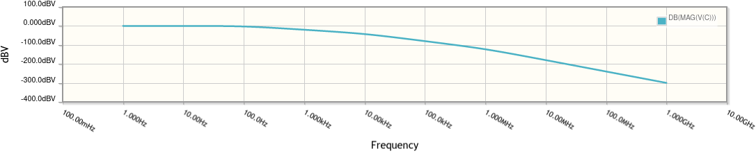
There is a flat region from DC, followed by a -20 dB/decade region, then a -40 dB/decade region, and finally a -60 dB/decade region.
The phase plot is where things get interesting. In the old version of CircuitLab, the phase plot looked like this:
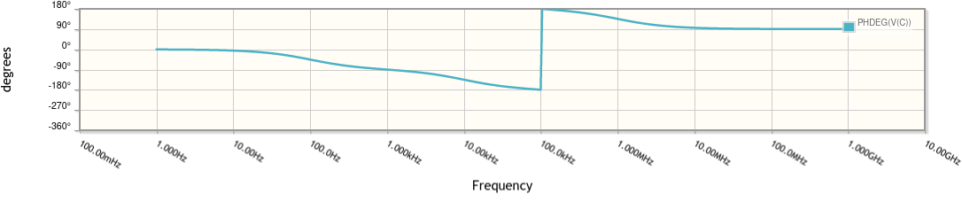
Notice that at around the 100 kHz point, the phase jumps from $-180^\circ$ to $+180^\circ$. This is a consequence of phase wrapping, rather than anything actually happening in the circuit above. The point on the complex plane has simply wrapped around.
In the new version of CircuitLab with phase unwrapping, the phase plot looks like this:
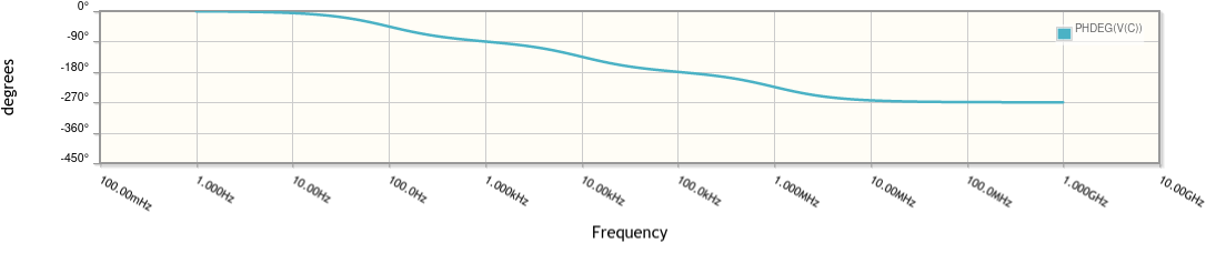
The unwrapped phase makes it more clear that each LPF adds $-90^\circ$ of phase lag. This is easier to understand, even if there’s no real difference between $-270^\circ$ and $+90^\circ$ of phase offset for a continuous sine wave.
Instead of using artificial (but convenient) Laplace Blocks, let’s build a real circuit, for example an AC-coupled analog amplifier using a NPN BJT:
Click the circuit above and run the frequency domain simulation for yourself. Feel free to change the circuit and see how the plot changes. For example, make C1 10x bigger or 10x smaller than it is now and re-run the simulation.
Again, the magnitude plot looks the same in both old and new versions of CircuitLab:
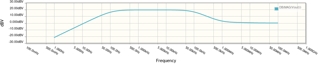
This amplifier gives about 10x voltage gain (+20 dB; see Orders of Magnitude, Logarithmic Scales, and Decibels) over a range of about 500 Hz to 50 kHz. The gain declines on either side of this range.
The phase plot is interesting too. In the old version of CircuitLab, the phase wrapped around and looked like this:
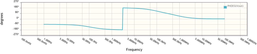
Note that the phase in the passband is right around $-180^\circ$. That’s because this is an inverting amplifier configuration. A small step up in the input causes a step down in the output.
In the new version of CircuitLab with phase unwrapping, the phase plot looks like this:
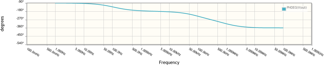
With phase unwrapping, it’s much easier to see that phase is relatively flat in the passband.
Eventually, at very high frequencies, the gain drops to 1 (+0 dB) and the phase drops to $-360^\circ$ (equivalent to zero). Basically, at very high frequencies, the capacitances in the circuit (specifically C1 and the base-collector capacitance $C_\mu$ of Q1) increasingly act like short circuits, and a small step up in the input causes an equally-sized step up in the output.
While there is no physical difference between a phase of $-185^\circ$ and $+175^\circ$, the discontinuity in the wrapped phase graphs made CircuitLab hard to use for frequency domain analysis.
This is especially true because there is often special interest in what’s happening from a feedback and circuit stability standpoint around the $\pm 180^\circ$ transition, or when analyzing circuits that naturally have inverting behavior in the frequency range of interest.
By modifying our complex number representation to have an integer wrap count, CircuitLab now unwraps the phase for the convenience of our users. In addition to adding new unit tests to our ComplexNumber class around this new behavior, the example circuits above are also part of our extensive integration test suite which we run whenever we modify the simulation engine to ensure we don’t inadvertently cause any behavior regressions as we continue to extend the software.
|
Brilliant. Thanks for this update. |
April 21, 2021 |
Please sign in or create an account to comment.
CircuitLab is an in-browser schematic capture and circuit simulation software tool to help you rapidly design and analyze analog and digital electronics systems.