In the screenshots below you'll learn how to use custom parameter elements to model and simulate a Pt100 RTD temperature sensor. CircuitLab's programming language-like features allow you to mix circuits and code, a more powerful combination than either alone.
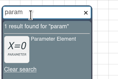
Press / (forward slash) to begin a toolbox search and type "param" to find the Parameter Element:
Click and drag to insert the element on to your schematic. Double-click to configure it:
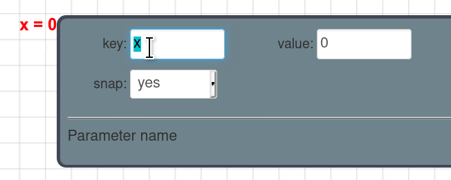
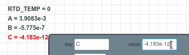
Type "RTD_TEMP" as the Key and leave "0" as the Value:
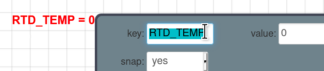
RTD_TEMP will be our independent variable, representing the temperature of our Pt100 RTD sensor in degrees Celsius.
Drag three more Parameter Elements from the toolbox onto the circuit and line them up below RTD_TEMP:
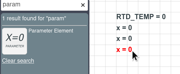
We'll use these three to define some constant values. Double-click each and type in the Key and Value fields to set A=3.9083e-3, B=-5.775e-7, and C=-4.183e-12:
These values describe the first, second, and third order variation in resistance of a platinum resistance thermometer with temperature. (See Wikipedia's Callendar-Van Dusen equation page for more detail.)
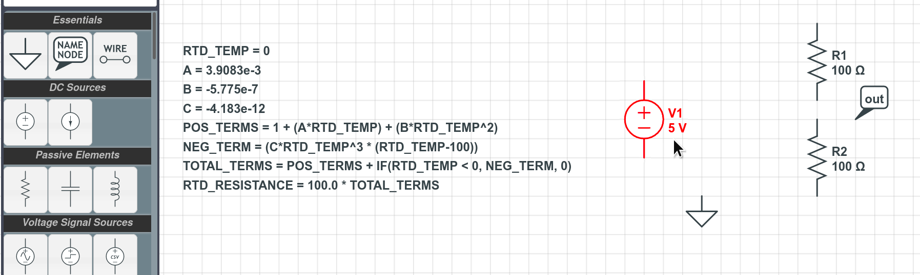
Next, we'll implement the equations. Drag in four more parameter elements, and set them as follows:
POS_TERMS="1 + (A*RTD_TEMP) + (B*RTD_TEMP^2)"
NEG_TERM = "(C*RTD_TEMP^3 * (RTD_TEMP-100))"
TOTAL_TERMS="POS_TERMS + IF(RTD_TEMP < 0, NEG_TERM, 0)"
RTD_RESISTANCE="100.0 * TOTAL_TERMS"
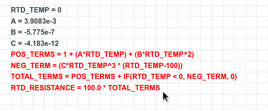
Parameters can reference other parameters by name, and can do math and even evaluate logic like IF statements.
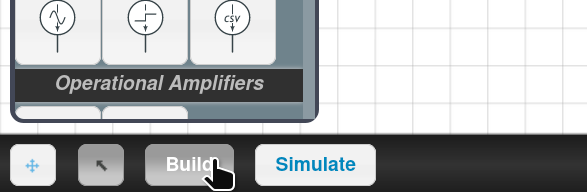
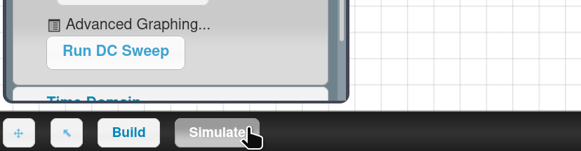
To see if this worked, click Simulate at the bottom of the window, and then click DC Sweep:
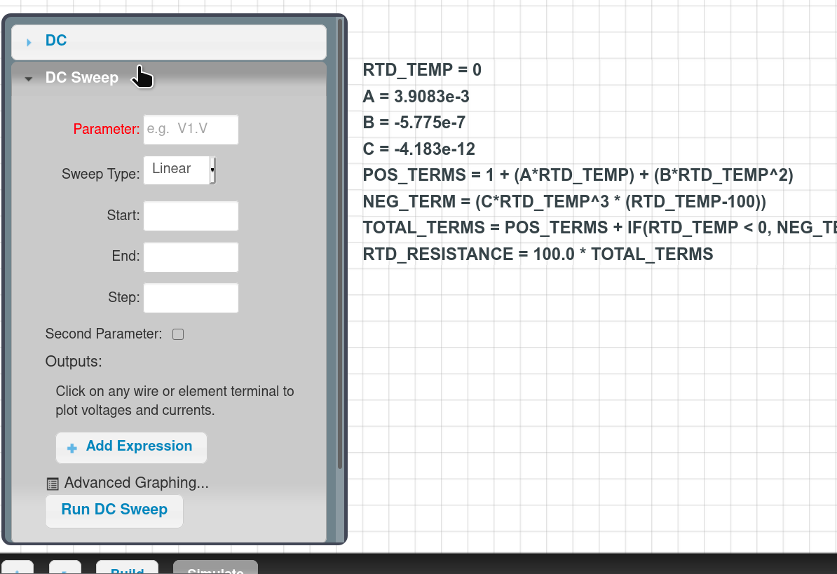
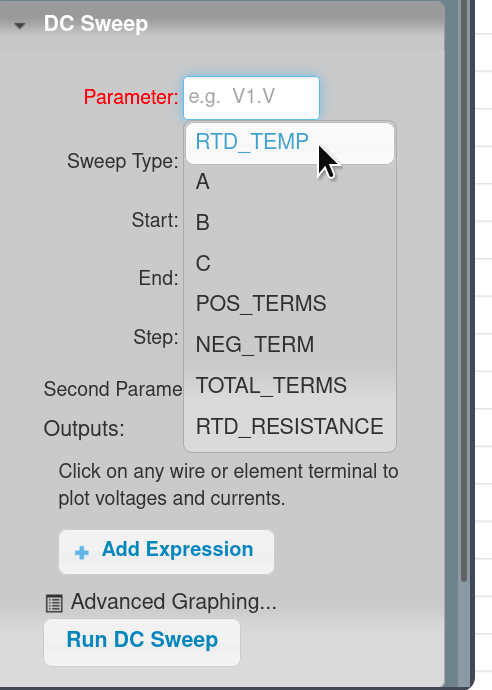
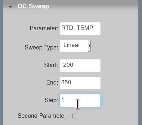
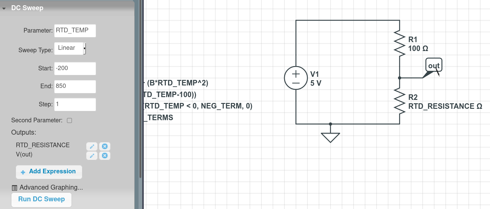
Click in the Parameter box and an autocomplete appears. Click RTD_TEMP to choose it as our independent variable:
Leave Sweep Type as Linear, and set Start to "-200" and End to "850", with a Step of "1":
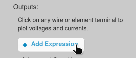
Under Outputs, click + Add Expression:
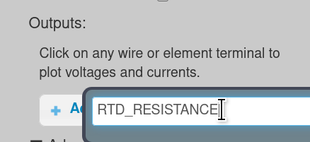
A text field appears asking what we'd like to plot. Type "RTD_RESISTANCE", indicating that we'd like the simulator to simply evaluate that parameter as our result variable, and press Enter:
This is now added to our Outputs list:
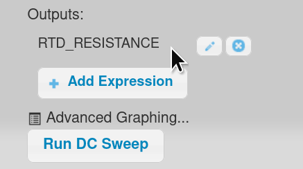
Click Run DC Sweep. A plot window appears:
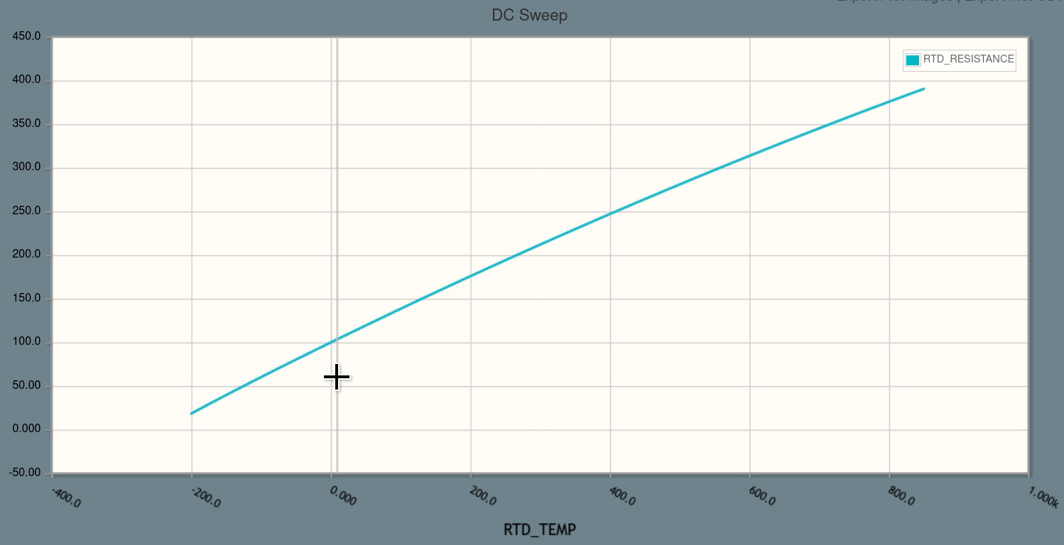
Success! We have temperature on the x-axis and resistance on the y-axis. We can quickly confirm that at RTD_TEMP=0, the Pt100 sensor's resistance is 100 ohms, and we can check a few other points on a table to confirm that we've properly implemented the equations.
Next, let's build a circuit using this RTD model. Click Build at the bottom of the window to return to build mode:
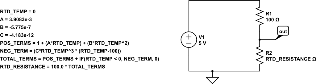
From the toolbox, click and drag on a voltage source, two resistors, a ground, and a node name. Then double-click on NODE1 and set the node name to "out", and double-click to make the voltage source be 5 volts:
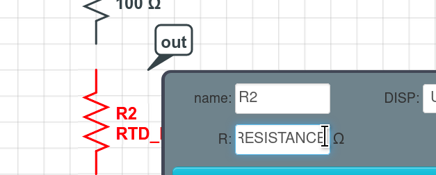
Now, let's make resistor R2 be controlled by our RTD_RESISTANCE parameter, rather than being a fixed 100 Ohms. Double-click R2 and type "RTD_RESISTANCE" in its R field:
Click and drag wires from the component terminals to finish wiring up the circuit so we have a voltage divider between R1 and R2, with V(out) connected at the voltage divider’s midpoint:
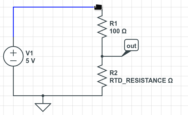
We're done building the circuit! This "out" node might be connected to an analog-to-digital converter (ADC) if we're interested in measuring the temperature, for example. Let's see how its voltage varies with the sensor's temperature.
Click Simulate at the bottom of the window:
Click on the node name "out" and notice that V(out) is added to our DC Sweep's Outputs list:
Click Run DC Sweep. A plot window appears:
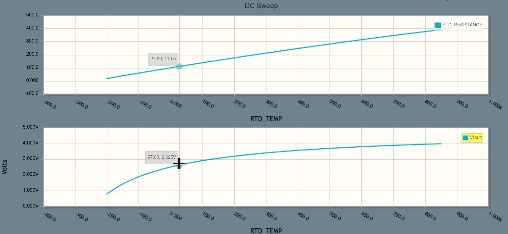
Perfect! In the bottom subplot, we can see how the V(out) voltage our ADC sees would vary with the sensor's temperature.
It's possible that we could design a better RTD measurement circuit than a simple voltage divider, but an engineer would almost certainly start with this simplest possible circuit first and then examine ways to improve it. (For example, 4-wire measurement to eliminate the effect of lead resistance, or better rejecting variations in the power supply voltage.)
That's it! Custom parameters are powerful tools for controlling your circuit simulations.
Click below to open the final circuit, or try it yourself from scratch (recommended).
CircuitLab is an in-browser schematic capture and circuit simulation software tool to help you rapidly design and analyze analog and digital electronics systems.